 First
let's look at the instrumented golf club.
First
let's look at the instrumented golf club.The TT engineers attached four strain gauges to the shaft at 90º intervals. A strain gauge is a device whose electrical properties change when it is stretched or compressed. When a shaft bends, the outside of the bend gets longer and the inside gets shorter. So a strain gauge on the outside of the bend will experience stretching, and one on the inside of the bend will experience compression.
The strain gauges on a ShaftLab club are arranged so that two measure lead-lag bend (the red ones in the picture) and the other two measure toe-heel bend (the green ones; only one is visible, the other being hidden behind the shaft). For instance, if the shaft experiences "lead" bend, the red strain gauge on the left is compressed and the one on the right is stretched. This produces an electrical differential that is sent to the computer.
How is the signal sent to the computer. So far (as of 2007), the club is tethered to the computer by a flexible cable. There have been many user requests to use some sort of wireless technology, but so far TT has not seen fit to do the modification.
So the computer gets two sets of signals from the golf club: the amount of lead-lag bend, and the amount of toe-heel bend.
It "sees" the bend as a point on two-dimensional graph. For instance, the red triangle in the X-Y graph at the left represents a bend that is considerably toe-up and somewhat lagging.
The computer's job is to save these points often enough to give a smooth curve of the bend during the swing. I think they sample every millisecond, but it may be every 2 milliseconds. The result is that the computer can plot the shaft bend variation with time for as much of the swing as you'd like. As the software comes from TT, the plot is designed to cover the downswing and looks like this....
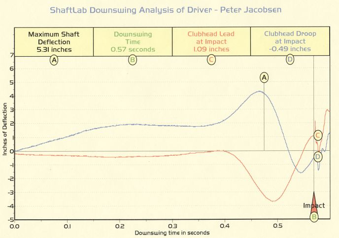
We can see from the graph that Jacobsen has a fairly long downswing: about 570 milliseconds from start to impact. (Later we will learn this isn't exactly true.) If we didn't read this from the graph, we could see it at the top of the page, where the software tabulates a few important parameters of the swing.

While this form of plot is certainly interesting, there is another plot that is at least as informative, that doesn't come with the ShaftLab software. (I used the Excel spreadsheet's plotting capability to generate it from the ShaftLab graph for Jacobsen.)
The graph at the right is a time-lapse picture of the X-Y plot we saw earlier on this page. The blue numbers next to the X-Y points are the milliseconds before impact. So we are tracing the two bends -- toe-heel and lead-lag -- for the 570 milliseconds of Jacobsen's downswing. A few points worth noting, which are typical characteristics of a pro swing:
- The first 400msec of the swing (more than 2/3 of the downswing), all the bend is toe-up, with very little lead-lag bend at all.
- The swing then turns into the [Toe-up, Lag] quadrant of the graph.
- With a little less than 100msec left to impact, the total bend peaks, a combination of toe-up and lag bend.
- For only the last 50msec do we see the bend get to toe-down, then show some lead. The actual direction of bend here is very chaotic. We will go into the reasons below, but you can also see this from the canonical ShaftLab output graph above.

